This blog post dissects the popular paper titled “Low-Resource” Text Classification: A Parameter-Free Classification Method with Compressors.
Author
Lennard Berger
Published
August 11, 2023
Some weeks ago I stumbled across one paper in particular titled: “Low-Resource” Text Classification: A Parameter-Free Classification Method with Compressors”(see Jiang et al. 2023). This paper has been dubbed the “gzip paper”, and has been largely discussed in the NLP community because of a refreshingly simple and efficient take on text classification. In the authors words they are matching neural networks in performance:
There have been several studies in this field (Teahan and Harper 2003); (Frank et al. 2000), most of them based on the intuition that the minimum cross entropy between a document and a language model of a class built by a compressor indicates the class of the document. However, previous works fall short of matching the quality of neural networks.
Some theory
As outlined in the quote above, one could regard text classification as a maximisation problem rather than a learning problem. This makes intuitive sense because of two reasons:
language usually follows a Zipf distribution (see Piantadosi 2014)
in a text classification problem different categories fall into different word registers
If we account for the fact that the top 10% of words are common words, it follows that there will be a number of distinct words and phrases which capture the “gist” of every category. For this idea to work, we are taking it as given our categories are distinct enough for a semantic differentiation.
For such datasets it appears unecessary to use a neural method, if all we truly want is to classify text. Taking this intuition further, the authors formulate two properties of compression algorithms, and how they can be exploited for text classification:
compressors are good at capturing regularity
objects from the same category share more regularity than those from different categories
To this end they derive the normalised compression distance from Bennet’s information distance (see Bennett et al. 1998) as follows:
As the normalised compression distance is tractable, we can compute the distance matrix for a given dataset in \(\mathcal{O}(n^2)\). This is mathematically elegant and simple, albeit not computationally efficient (it could be improved by employing caching on the compressor).
Reproduction
The authors made reproduction easy for us because they kindly added a Python implementation. For the sake of this blogpost I adjusted the code and divided into computation and analysis step respectively. To reproduce the paper I decided to use the 20newsgroups dataset also present in the paper. This is mainly for four reasons:
it is available out of the box via scikit-learn which is convenient
it is well-known and established benchmark dataset on a variety of tasks
20newsgroups is a low-resource dataset (which is hard to begin with)
the size of the dataset makes it feasible for me to compute on my local machine without much hassle
The first step after computation is evaluation, so we’ll jump to that:
Code
from IPython.display import display, HTMLfrom sklearn.datasets import fetch_20newsgroupsfrom sklearn.metrics import classification_reportimport numpy as npimport seaborn as snsimport matplotlib.pyplot as pltimport pandas as pddataset_train = fetch_20newsgroups(subset='train', random_state=123)dataset_test = fetch_20newsgroups(subset='test', random_state=123)compressed_train_set = np.load("20newsgroups.train.npy")compressed_test_set = np.load("20newsgroups.test.npy")ncd = np.load("20newsgroups.ncd.npy")k =2y_pred = []for index inrange(len(ncd)): sorted_idx = np.argsort(ncd[index, :]) top_k_class = dataset_train["target"][sorted_idx[:k]].tolist() predict_class =max(set(top_k_class), key=top_k_class.count) y_pred.append(predict_class)ncd_report_df = pd.DataFrame(classification_report(dataset_test["target"], y_pred, target_names=dataset_test["target_names"], output_dict=True))display(HTML(ncd_report_df.to_html()))
Table 1: Classification report for normalised compressed distances on the 20newsgroups dataset
alt.atheism
comp.graphics
comp.os.ms-windows.misc
comp.sys.ibm.pc.hardware
comp.sys.mac.hardware
comp.windows.x
misc.forsale
rec.autos
rec.motorcycles
rec.sport.baseball
rec.sport.hockey
sci.crypt
sci.electronics
sci.med
sci.space
soc.religion.christian
talk.politics.guns
talk.politics.mideast
talk.politics.misc
talk.religion.misc
accuracy
macro avg
weighted avg
precision
0.561404
0.313002
0.363071
0.338809
0.441860
0.612335
0.699552
0.835294
0.595782
0.506986
0.665049
0.633110
0.476190
0.630631
0.791667
0.945017
0.537313
0.706329
0.621622
0.559471
0.559081
0.591725
0.592931
recall
0.802508
0.501285
0.444162
0.420918
0.394805
0.351899
0.400000
0.358586
0.851759
0.639798
0.686717
0.714646
0.407125
0.353535
0.578680
0.690955
0.791209
0.742021
0.593548
0.505976
0.559081
0.561507
0.559081
f1-score
0.660645
0.385375
0.399543
0.375427
0.417010
0.446945
0.508972
0.501767
0.701138
0.565702
0.675709
0.671412
0.438957
0.453074
0.668622
0.798258
0.640000
0.723735
0.607261
0.531381
0.559081
0.558547
0.557414
support
319.000000
389.000000
394.000000
392.000000
385.000000
395.000000
390.000000
396.000000
398.000000
397.000000
399.000000
396.000000
393.000000
396.000000
394.000000
398.000000
364.000000
376.000000
310.000000
251.000000
0.559081
7532.000000
7532.000000
At 0.59 weighted average precision the algorithm significantly underperforms compared to the paper (reported with 0.685). However, such artefacts are not uncommon, and there are a variety of factors (such as the operating system) which can affect compression. The results are in the same ballpark, and 0.59 precision is still fairly decent, given this is a pure computational approach to classifying 20 categories.
mode knn vs weighted
The default implementation of the paper uses mode to assign the class with the highest probability. This is odd in two ways.
Firstly it obscures the benchmark (why use a non-standard behaviour?). Secondly,it probably makes the benchmark harder, because often the weighted knn outperforms mode.
Inspecting the normalised compression distance
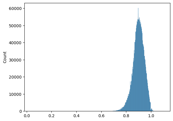
Since the authors claim their distance is a normalised distribution one would like to make sure this claim is correct. Typically a plot helps.
Table 2: Normaltest result for normalised compressed distance matrix
statistic
pvalue
767182.369619
0.0
Beyond doubt the NCD is of a normal distribution. Our next step is inspecting the input data from which the NCD is derived.
Code
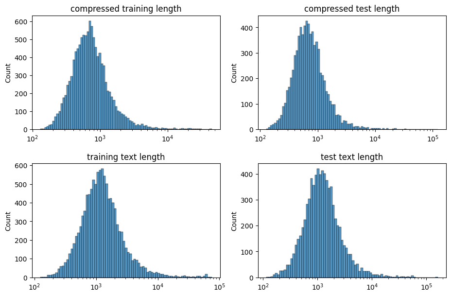
fig, (ax1, ax2, ax3, ax4) = plt.subplots(nrows=1, ncols=4,figsize=(11, 7))grid = plt.GridSpec(2, 2, wspace=0.2, hspace=0.3)ax1 = plt.subplot(grid[0, 0])ax2 = plt.subplot(grid[0, 1:])ax3 = plt.subplot(grid[1, :1])ax4 = plt.subplot(grid[1, 1:])sns.histplot(compressed_train_set, log_scale=True, ax=ax1)sns.histplot(compressed_test_set, log_scale=True, ax=ax2)sns.histplot([len(x2) for x2 in dataset_train["data"]], log_scale=True, ax=ax3)sns.histplot([len(x1) for x1 in dataset_test["data"]], log_scale=True, ax=ax4)ax1.title.set_text("compressed training length")ax2.title.set_text("compressed test length")ax3.title.set_text("training text length")ax4.title.set_text("test text length")plt.show()
/var/folders/k6/hdzmrkf915d0twbr_qmhy9l00000gn/T/ipykernel_69344/1604665436.py:8: MatplotlibDeprecationWarning: Auto-removal of overlapping axes is deprecated since 3.6 and will be removed two minor releases later; explicitly call ax.remove() as needed.
  ax1 = plt.subplot(grid[0, 0])
/var/folders/k6/hdzmrkf915d0twbr_qmhy9l00000gn/T/ipykernel_69344/1604665436.py:9: MatplotlibDeprecationWarning: Auto-removal of overlapping axes is deprecated since 3.6 and will be removed two minor releases later; explicitly call ax.remove() as needed.
  ax2 = plt.subplot(grid[0, 1:])
Figure 2: Histograms of training and test lengths (un)compressed
This finding may not be a surprise to everyone, but it is highly interesting. If the NCD is derived from the compressed length, and the text length is of the identical distribution as the compressed length, we should be able to simplify this model.
Encoding linguistic knowledge into our model
Few things will sour linguists as much as researchers trying to build models (and algorithms), deliberately ignoring domain knowledge. In this sense, let’s help with some insights from the linguistics department.
If the text length and compressed length are of the same distribution, the standard approach is to use a bag-of-word model. We could (computationally) simplify the NCD significantly. To do so:
build a simple CountVectorizer model
create a count matrix for the training and test data set
calculate the normalised count distance
reevaluate
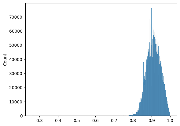
Just as with the original paper, it is possible to split the code into computation and analysis. Using the computed count matrix, first we evaluate wether the count matrix and the original NCD are indeed of the same distribution.
Our intuition is spot on. This distribution plot is very similar to the one of the original NCD, to say the least. A mood test can help us determine if the scales are indeed identical.
Code
res = stats.mood(sample, sample_count)ncd_mood_test_df = pd.DataFrame([[res.statistic.tolist(), res.pvalue.tolist()]], columns=["statistic", "pvalue"])display(HTML(ncd_mood_test_df.to_html(index=False)))
Table 3: Mood test result for normalised compressed distance matrix and normalised count distance matrix
statistic
pvalue
387.040639
0.0
Now that we can produce equivalent NCD values from counts, we can reevaluate the original model.
Table 4: Classification report for normalised count distances on the 20newsgroups dataset
alt.atheism
comp.graphics
comp.os.ms-windows.misc
comp.sys.ibm.pc.hardware
comp.sys.mac.hardware
comp.windows.x
misc.forsale
rec.autos
rec.motorcycles
rec.sport.baseball
rec.sport.hockey
sci.crypt
sci.electronics
sci.med
sci.space
soc.religion.christian
talk.politics.guns
talk.politics.mideast
talk.politics.misc
talk.religion.misc
accuracy
macro avg
weighted avg
precision
0.408621
0.323248
0.363265
0.392202
0.418301
0.597633
0.796117
0.788462
0.497703
0.443015
0.626289
0.567227
0.390476
0.601852
0.807692
0.871795
0.462057
0.680217
0.546468
0.403704
0.505975
0.549317
0.554029
recall
0.742947
0.521851
0.451777
0.436224
0.332468
0.255696
0.420513
0.310606
0.816583
0.607053
0.609023
0.681818
0.312977
0.328283
0.479695
0.512563
0.752747
0.667553
0.474194
0.434263
0.505975
0.507442
0.505975
f1-score
0.527253
0.399213
0.402715
0.413043
0.370478
0.358156
0.550336
0.445652
0.618459
0.512221
0.617535
0.619266
0.347458
0.424837
0.601911
0.645570
0.572623
0.673826
0.507772
0.418426
0.505975
0.501337
0.502325
support
319.000000
389.000000
394.000000
392.000000
385.000000
395.000000
390.000000
396.000000
398.000000
397.000000
399.000000
396.000000
393.000000
396.000000
394.000000
398.000000
364.000000
376.000000
310.000000
251.000000
0.505975
7532.000000
7532.000000
With 0.55 weighted average precision we lost 4 points to the original NCD. Interestingly, the recall values for individual categories are very similar.
Interim result
We can build an approximately similar model to NCD using CountVectorizer. However, our linguistic model has a few distinct advantages:
It is extremely fast (NCD is computed in ~30 minutes on 8 threads, counts are computed in 5 minutes with 1 thread)
CountVectorizer can generalise better to unseen data because of the Zipfian law
We have yet to start with other domain tricks such as preprocessing, which will boost the result
That’s fair enough, you say, but simply building out a model is not sufficient.
One of the major points the authors of the gzip paper emphasize is explainability. While explainability in neural architectures is tricky at best, the NCD is only mathematically explainable. For us mere humans, we still don’t know what this model actually encodes. That’s where CountVectorizer can come to our rescue.
What’s our KNN actually predicting?
Turning back to the authors original idea, we can speculate that:
The most common words will be stripped by compression
There are low-frequency words associated with the different categories
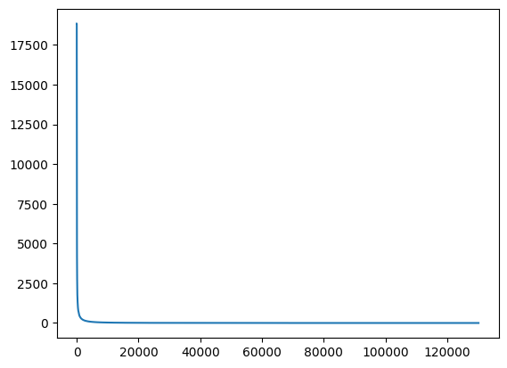
To prove this, we can inspect the count vectorizer. First, we will take a look at the token distribution:
Code
from collections import Counterfrom sklearn.feature_extraction.text import CountVectorizervectorizer = CountVectorizer()train_dataset_count = vectorizer.fit_transform(dataset_train["data"])test_dataset_count = vectorizer.transform(dataset_test["data"])# nonzero indexes represents where data is actually storedindex_counter = Counter(train_dataset_count.nonzero()[1].tolist() + test_dataset_count.nonzero()[1].tolist())fig, ax = plt.subplots()sns.lineplot([count for idx, count in index_counter.most_common()], ax=ax)plt.show()
Figure 4: Histogram of token counts in 20newsgroup dataset
Yep, that’s a Zipfian distribution! If we discard the most common terms from this dataset, we can try and correlate it with our categories. To do so, we run the spearman correlation between the categories and the decomposition of the remaining matrix.
Table 5: Spearman correlation coefficient for 1-D decomposition of the 20newsgroups dataset
statistic
pvalue
0.264924
5.053535e-181
Would you look at this. A slight positive correlation with significance! With this knowledge at hand, we can note down how NCD works.
If there are sufficient uncommon words per category, NCD boosts the likelihood per category by maximising infrequent terms.
This approach may fall flat if categories consist of very similar words (such as is the case in humour detection).
Closing remarks
Recently there has been a strong trend with the sentiment: “neural architectures solves everything”. In the light of this, I find it admirable to seek ways to efficiently model simple problems.
However, there is a decent amount of evidence showing that neural architectures are not the sole source of improvements in the field of NLP. Preprocessing is of particular importance to all kinds of models, notwithstanding neural architectures (see Levy et al. 2015).
In this regard the gzip paper falls short. Preprocessing isn’t a tiresome step of modelling, it is actually our single best friend to combat sparseness.
References
Bennett, C. H., P. Gacs, Ming Li, P. M. B. Vitanyi, and W. H. Zurek. 1998. “Information Distance.”IEEE Transactions on Information Theory 44 (4): 1407–23. https://doi.org/10.1109/18.681318.
Frank, Eibe, Chang Chui, and Ian H Witten. 2000. Text Categorization Using Compression Models.
Jiang, Zhiying, Matthew Yang, Mikhail Tsirlin, Raphael Tang, Yiqin Dai, and Jimmy Lin. 2023. “‘Low-Resource’ Text Classification: A Parameter-Free Classification Method with Compressors.”Findings of the Association for Computational Linguistics: ACL 2023, 6810–28.
Levy, Omer, Yoav Goldberg, and Ido Dagan. 2015. “Improving Distributional Similarity with Lessons Learned from Word Embeddings.”Transactions of the Association for Computational Linguistics (Cambridge, MA) 3: 211–25. https://doi.org/10.1162/tacl_a_00134.
Piantadosi, Steven T. 2014. “Zipf’s Word Frequency Law in Natural Language: A Critical Review and Future Directions.”Psychonomic Bulletin & Review 21: 1112–30.
Teahan, William J, and David J Harper. 2003. “Using Compression-Based Language Models for Text Categorization.”Language Modeling for Information Retrieval, 141–65.