Building a property graph database from scratch
As can be seen from the featured image above, many natural processes can be modeled as graphs. Transactions of individuals in a payment network are classic datasets for which graphs are a natural fit. Once such a dataset is loaded into a graph we can easily answer questions such as:
- how many steps does an average transaction take?
- who is a 2nd-level collaborator of “x”?
These questions could be answered from a relational database. However, modeling relational databases is not intuitive (for the problem), and in many cases not very performant. It is for this reason, that graph databases have steadily gained popularity, especially in the area of knowledge graphs.
This blog post will give an introduction to the concepts underlying a “Labeled-property graph”, which is the most widely used type of graph representation available today. Labeled-property graphs are commonly defined like below:
A labeled-property graph model is represented by a set of nodes, relationships, properties, and labels. Both nodes of data and their relationships are named and can store properties represented by key-value pairs. Nodes can be labeled to be grouped. (Wikipedia 2024)
Back to the basics
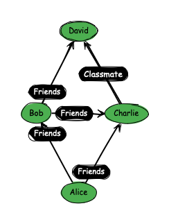
Before we dive head-deep into implementation, we should take a moment to review the basics of graphs. In the simplest form, a graph consists of:
- nodes (Bob, David, Charlie and Alice)
- edges (Friends, Classmate)
Two nodes are connected by an edge. We call these two nodes adjacent. Graphs can be directional (as in our class of students example) or undirected. Some implementations even allow for mixed graphs. This depends on your use case. A friendship network would more likely be represented as an undirected network because friendship is a transitive relationship. This blog post will focus on undirected networks, as they are easier to implement, all the while representing the fundamental properties underlying all graphs.
Finding a path
If one wants to know how many friends and friends-of-friends Alice has, they need to ask Alice, and all her friends respectively. In terms of graph networks, this process is called traversal. There are two main kinds of traversal algorithms:
- depth-first search, visits children of nodes before siblings
- breadth-first search, visits siblings of nodes before children (can be useful for finding the shortest path to x)
For the sake of simplicity, we will use a depth-first search in this article. It is the most intuitive to implement and evaluate. To gain an intuitive understanding of the algorithm, it can be helpful to illustrate the problem. In the following animation, a depth-first traversal algorithm is shown. Blue indicates the start node whereas red indicates the end node the algorithm uses for every step, respectively. Green nodes are not considered in that step.

There are much more comprehensive resources, such as (Even 2011), explaining traversal in-depth. In this blog post, we will take DFS as a given, and use it for our implementation.
Representing graphs
We solved the first graph problem, which is graph traversal. To make a graph database, we will also need to store our graph. A simple and effective way is a so-called adjacency list. In an adjacency list, we store one list per node (which we call source). In this list, we store the target nodes. It is as simple as this. The definition of our example graph could be written like so:
Alice Bob Charlie
Bob Charlie David
Charlie David
Here:
Aliceis the source of two edges, one toBoband one toCharlieBobis the source of two edges, one toCharlieand one toDavidCharlieis the source of one edge toDavid
Adjacency lists are very compact, yet efficient representations of graphs (both in storage and computation). For small graphs, an adjacency matrix (where every node is represented in a \(N \times N\) matrix) can be even faster (for lookups). As adjacency matrices require \(O(n^2)\) in storage capacity, they are not very popular for implementations. Thus, we will focus on adjacency lists.
First graph database implementation
With both traversal and storage for our graph database solved, we can move on to the first version of our implementation.
Since we are not interested in dealing with all the complexities of a fully-fledged database (such as consistency guarantees), we can start by leveraging an existing database. One simple, yet extremely powerful database that comes pre-installed on many platforms, is SQLite. In this example, we will build our graph database powered by SQLite. The first step is to create the table definition for our graph. Borrowing from the definition of the adjacency list, we could define our table like so:
CREATE TABLE edge(source TEXT, target TEXT);
CREATE INDEX edge_source ON edge(source);
CREATE INDEX edge_target ON edge(target);
As SQLite is a powerful database, this is all that is necessary to store our graph, as well as traverse it. A traversal query can be achieved using a WITH statement:
WITH RECURSIVE nodes(x) AS (
   SELECT "Alice"
   UNION
   SELECT source FROM edge JOIN nodes ON target=x
   UNION
   SELECT target FROM edge JOIN nodes ON source=x
)
SELECT x FROM nodes;
Adding properties
You may have noticed our implementation is lacking the properties of a labeled-property graph. To support labels, we can extend our existing definition. To do so, we extend the edges table:
CREATE TABLE edge(source TEXT NOT NULL, target TEXT NOT NULL, label TEXT);The edge label has now become a SQLite TEXT field, which allows us to write many flexible queries.
Putting it all together
As we have a traversal algorithm, graph database storage and the labels of our property-labeled graph available, we can write an implementation that leverages all of this. To do so, we will write a small command-line application. Our application should have the following features:
- create a database file from an adjacency list and a list of edge labels
- allow querying of the graph (which nodes are reachable from “x”)
- incorporate the property graph (who are friends of friends of Alice?)
For starters, let’s write a command to initialize the database. This script should read an adjacency list file, and optionally a labels file, with one label per edge:
import sqlite3
from pathlib import Path
from typing import Optional

def init_database(
        adjacency_list_file: Path,
        output_database_file: Path,
        labels_file: Optional[Path] = None
):
    """
    Reads an adjacency list file and creates a graph database from it.
    If a labels file is supplied, it is read and the labels for the edges are created in insertion order.

    :param adjacency_list_file: The adjacency list to read.
    :param output_database_file: The output database file.
    :param labels_file: An optional edge label file.
    """

    sources, targets = [], []

    with adjacency_list_file.open() as fp:
        for line in fp:
            edges = line.split(" ")
            source = edges[0].strip()

            for target in edges[1:]:
                sources.append(source)
                targets.append(target.strip())

    if labels_file is not None:
        with labels_file.open() as fp:
            labels = [line.strip() for line in fp.readlines()]

            if len(labels) != len(sources):
                raise ValueError(f"Trying to map {len(labels)} onto {len(sources)} edges!")

    con = sqlite3.connect(output_database_file)
    cur = con.cursor()

    cur.executescript("""
        CREATE TABLE edge(source TEXT NOT NULL, target TEXT NOT NULL, label TEXT);
        CREATE INDEX edge_source ON edge(source);
        CREATE INDEX edge_target ON edge(target);
    """)

    con.commit()

    query = "INSERT INTO edge(source, target, label) VALUES (?, ?, ?)" if labels_file is not None else "INSERT INTO edge(source, target) VALUES (?, ?)"
    edges = zip(sources, targets, labels) if labels_file is not None else zip(sources, targets)

    cur.executemany(query, edges)
    con.commit()
Next, we want to implement a simple query by specifying the start node for our inquiry. We can implement a command to give back all the nodes satisfying our request:
def query(output_database_file: Path, node: str):
    """
    Reads a graph database and returns all nodes reachable from the given node.

    :param output_database_file: The graph database to read.
    :param node: The start node.
    :return: A list of nodes reachable from the start node.
    """

    con = sqlite3.connect(output_database_file)
    cur = con.cursor()
    res = cur.execute("""
    WITH RECURSIVE nodes(x) AS (
        SELECT ?
        UNION
        SELECT source FROM edge JOIN nodes ON target=x
        UNION
        SELECT target FROM edge JOIN nodes ON source=x
    )
    SELECT x FROM nodes;
    """, (node.strip(),))
    targets = res.fetchall()

    print(f"Nodes that can be reached from {node.strip()}")
    print(targets)
This allows us to query the graph in a depth-first approach. E.g running the query for “Alice”, we’d get:
Nodes that can be reached from Alice
[('Alice',), ('Bob',), ('Charlie',), ('David',)]
As a final step, we can incorporate a filter for our labels:
if label is not None:
   res = cur.execute("""
   WITH RECURSIVE nodes(x) AS (
      SELECT ?
      UNION
      SELECT source FROM edge JOIN nodes ON target=x WHERE label LIKE ?
      UNION
      SELECT target FROM edge JOIN nodes ON source=x WHERE label LIKE ?
   )
   SELECT x FROM nodes;
   """, (node.strip(), label.strip(), label.strip(),))
else:
   res = cur.execute("""
   WITH RECURSIVE nodes(x) AS (
      SELECT ?
      UNION
      SELECT source FROM edge JOIN nodes ON target=x
      UNION
      SELECT target FROM edge JOIN nodes ON source=x
   )
   SELECT x FROM nodes;
   """, (node.strip(),))
This allows for precise queries of the edge label and wildcard usage. The fully-compiled script is attached to this blog post.
Real-world complexities
In this blog post, we have introduced the basic functionalities of a property-labeled graph:
- efficient data storage
- graph traversal
- labeled edge queries
However, in the real world, these are not sufficient. Many feature ideas come to mind here that we didn’t implement:
- support for node labels
- support for directed graphs
- more flexible properties (this could be done using SQLite’s JSON field)
Furthermore, querying our graph with SQL is inconvenient at best. It is for this reason that many mature graph databases exist. Solutions like Neo4j or JanusGraph implement support for many different graph paradigms (self-loops, directed-, undirected and mixed graphs), and much more convenient query capabilities. However, they will follow the same basic building blocks discussed in this blog post.