import numpy as np
from more_itertools import batched
def calculate_hist(file_name: str, chunk_size=100000, num_bins=100):
# Initialize empty arrays to store cumulative counts and bins
cumulative_counts = np.zeros(num_bins)
counts, bins = None, None
with open(file_name) as fp:
# Loop through the data in chunks
for lines in batched(fp, chunk_size):
distances = [1 - float(line.strip()) for line in lines]
counts, bins = np.histogram(distances, bins=num_bins)
cumulative_counts += counts
return counts, binsWord embedding similarity is tricky
python
rust
word embeddings
machine learning
Even though word embeddings are widely used, we do not know a whole lot about them

This post will be a deep dive into word embeddings. Word embeddings have made multiple appearances on this blog, such as in my talk about neural networks, or the spaCy benchmark. The reason I am captivated by word embeddings is threefold:
- they are very useful, the underlying building blocks for most text-based machine learning models
- word embeddings are computationally efficient (you can encode “all the language’s meaning” in a few hundred megabyte)
- very few people actually understand what the consequences of embeddings are
Cosine similarity is the most popular method to date to compare embeddings (such as in document retrieval). A recent paper by (Steck et al. 2024) investigated the usage of cosine similarity and uncovered some surprising findings:
We study cosine similarities in the context of linear matrix factorization models, which allow for analytical derivations, and show that cosine similarities are heavily dependent on the method and regularization technique, and in some cases can be rendered even meaningless.
The de-facto industry standard method doesn’t really work? It seems counterintuitive.
From my experience on working on retrieval augmented generation, I would say that does check out. Cosine similarity does convey a sense of similarity, but often times results are very counterintuitive.
To corroborate these suspicions, I thought it would be interesting to investigate two popular word embedding models:
- GloVe: Global Vectors for Word Representation (Pennington et al. 2014)
- Word2Vec (Bojanowski et al. 2016)
Making assumptions
To start an investigation, some assumptions will need to be made:
- for vocabulary of size \(N\), word embeddings should project a matrix of size \(N \times N\)
- for every item in the matrix, the cosine similarity should be \(\{-1, ..., 1\} \in ℝ\)
- thus, the expected mean of all similarities should be \(0\)
With these assumptions at hand, the next step is to obtain the embeddings we want to experiment with. GloVe vectors can be downloaded right from the Stanford website. They are stored in a simple format. Each line contains one word, and a list of floating point numbers seperated by space. For the word “the” this looks like so:
the 0.04656 0.21318 -0.0074364 -0.45854 ...One can download pre-trained word2vec vectors from the fasttext website. However, they are not of the same format as GloVe, thus we should convert them to be more usable. We can do this with a few simple lines of Python:
import argparse
from pathlib import Path

from fasttext import FastText
import fasttext.util
from tqdm import tqdm


def write_model(output_file: Path, model: FastText):
    with output_file.open("wt") as fp:
        for word in tqdm(model.words):
            line_elements = [word] + [str(num) for num in ft.get_word_vector(word)]
            line = " ".join(line_elements)
            print(line, file=fp)


if __name__ == "__main__":
    parser = argparse.ArgumentParser()
    parser.add_argument("output_file", type=Path)
    args = parser.parse_args()

    ft = fasttext.load_model('cc.en.300.bin')
    write_model(args.output_file, ft)
Calculating a similarity matrix
Next, we want to calculate a similarity matrix for our words:
\(\forall word_1, word_2 \in vector: cos(word_1, word_2)\)
While theoretically simple, it turns out to be a non-trivial undertaking. Using simple multiplication we find the storage requirement for our embeddings to be:
- for GloVe, \(400000^2 * 4 / 10^{9} = 640 GB\)
- for fasttext, \(1000000^2 * 4 / 10^{11} = 4 TB\)
Simply saving the similarity matrices will require \(4.6\) terabyte of storage. Not ideal for a small experiment. Beyond storage space, we need to keep the runtime complexity in check. (Wenkel 2024) wrote a fast version of cosine distance in Rust, which we we will lend for this blog post:
pub fn cosine_dist_rust_loop_vec(vec_a: &[f64], vec_b: &[f64], vec_size: &i64) -> f64
{
    let mut a_dot_b:f64 = 0.0;
    let mut a_mag:f64 = 0.0;
    let mut b_mag:f64 = 0.0;

    for i in 0..*vec_size as usize
    {
        a_dot_b += vec_a[i] * vec_b[i];
        a_mag += vec_a[i] * vec_a[i];
        b_mag += vec_b[i] * vec_b[i];
    }

    let dist:f64 = 1.0 - (a_dot_b / (a_mag.sqrt() * b_mag.sqrt()));

    return dist
}
Thus, for every word, we will perform \(D*3 + 1\) multiplications where \(D\) is the dimensions of the vector. We will conclude that the runtime complexity of calculating the full similarity matrix is \(O(3N*D^2)\) operations (for the sake of argument, the other operations are negligible). This means:
- GloVe will require \((3*300*400000)^2 = 1.296*10^{17}\) multiplications
- fasttext will require \((3*300*1000000)^2 = 8.1*10^{17}\) multiplications
Which is a significant amount of operations. This should be an obvious reason why embeddings are not stored as similarity matrices. For the sake of simplicity, we will sample \(0.5\%\) of these similarities. For GloVe we will reduce our sample vocabulary to \(20000\) , whereas for fasttext it will be reduced to \(50000\) words.
Now, we can piece together a simple Rust program to calculate the cosine similarities for us. To do so, first we load the model into memory:
use std::collections::HashMap;
use std::fs::File;
use std::io::{BufRead, BufReader};
use std::path::Path;

pub type Embedding = HashMap<String, Vec<f64>>;


pub fn load_model(input_file: &Path) -> Result<Embedding, std::io::Error> {
    let mut model = HashMap::new();
    let file = File::open(input_file)?;
    let reader = BufReader::new(file);

    for line in reader.lines() {
        let line = line?;
        let items: Vec<String> = line.split_whitespace().map(|s| s.to_string()).collect();
        let word = items[0].clone();
        let embedding: Vec<f64> = items[1..]
            .iter()
            .map(|s| s.parse::<f64>())
            .collect::<Result<Vec<_>, _>>().unwrap();
        model.insert(word, embedding);
    }

    Ok(model)
}
Our load_model function returns a hashmap of every word to its respective vector.
Finally, we piece together our main function. It will iterate through all words in our hashmap, and write each distance to a file:
use std::fs::{OpenOptions};
use std::io::{LineWriter, Write};
use std::path::{Path, PathBuf};
use tqdm::pbar;
use embedding_network::{cosine_dist_rust_loop_vec, load_model};


fn write_distances(model_path: &Path, output_path: &Path) {
    let model = load_model(model_path).unwrap();
    let mut pbar = pbar(Some(model.len() * model.len()));
    let file = OpenOptions::new()
        .write(true)
        .create(true)
        .open(output_path).unwrap();
    let mut writer = LineWriter::new(file);

    for (_, vec1) in &model {
        for (_, vec2) in &model {
            pbar.update(1).unwrap();
            let distance = cosine_dist_rust_loop_vec(
                vec1,
                vec2,
                &(vec1.len() as i64)
            );

            writer.write_fmt(format_args!("{}\n", distance)).unwrap();
        }
    }

    writer.flush().unwrap();
}


struct Cli {
    input: PathBuf,
    output: PathBuf,
}

fn main() {
    let input_path = std::env::args().nth(1).expect("no input path given");
    let output_path = std::env::args().nth(2).expect("no output path given");

    let args = Cli {
        input: PathBuf::from(input_path),
        output: PathBuf::from(output_path),
    };

    write_distances(args.input.as_path(), args.output.as_path());
}
A full copy of the program is attached to this blog post.
Evaluating distances
Caution
In a previous iteration of this blog post, the cosine distance was accumulated in the histogram. After a hint by one of the attentive readers, the post has been updated accordingly.
Once we calculated the distances, we can read them out and plot a histogram. To measure the cosine similarity, we need to convert the distances accordingly: \(sim = 1 - dist\).
Since we have a lot of data, a simple plt.hist() would be really slow. Instead, we cumulate our data into a histogram:
counts_glove, bins_glove = calculate_hist("/Users/fohlen/RustRoverProjects/embedding_network/glove.6B.300d.distances.txt")
counts_fasttext, bins_fasttext = calculate_hist("/Users/fohlen/RustRoverProjects/embedding_network/cc.en.300.distances.txt")
Finally, we can plot our histogram:
import matplotlib.pyplot as plt

#| label: fig-hist-cosine-similarities-glove
#| fig-cap: "Histogram of similarities in GloVe 300d"

# Plot the histogram as bars
plt.bar(bins_glove[:-1], counts_glove)  # Use bins[:-1] to avoid plotting the upper bin edge twice

plt.xlabel("Cosine similarity")
plt.ylabel("Number of elements")

# Display the plot
plt.show()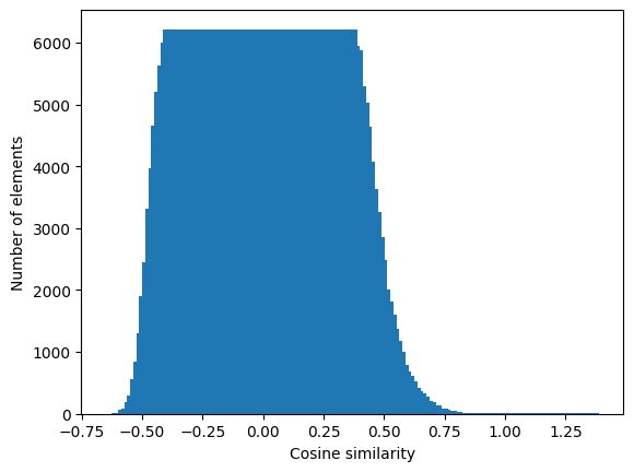
We repeat the same steps for our fasttext embeddings:
import matplotlib.pyplot as plt

#| label: fig-hist-cosine-similarities-fasttext
#| fig-cap: "Histogram of similarities in fasttext 300d"

# Plot the histogram as bars
plt.bar(bins_fasttext[:-1], counts_fasttext)  # Use bins[:-1] to avoid plotting the upper bin edge twice

plt.xlabel("Cosine similarity")
plt.ylabel("Number of elements")

# Display the plot
plt.show()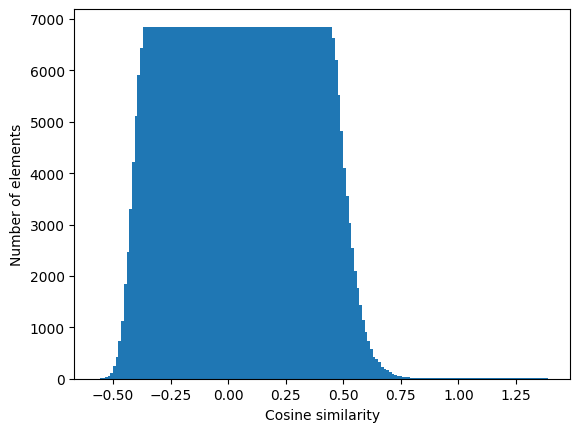
Results
To make better judgements, we should calculate the mean and standard deviation of our distributions:
import math

def weighted_avg_and_std(values, weights):
    """
    Return the weighted average and standard deviation.

    They weights are in effect first normalized so that they
    sum to 1 (and so they must not all be 0).

    values, weights -- NumPy ndarrays with the same shape.
    """
    average = np.average(values, weights=weights)
    # Fast and numerically precise:
    variance = np.average((values-average)**2, weights=weights)
    return (average, math.sqrt(variance))

print(weighted_avg_and_std(bins_glove[:-1], counts_glove))
print(weighted_avg_and_std(bins_fasttext[:-1], counts_fasttext))
(0.023056257271547205, 0.09445021476931395)
(0.06156012189878254, 0.0749758363367772)We can see that our assumptions hold up, as cosine similarity is a normal distribution with mean of \(\approx 0\). The standard deviation is seven to nine percent, depending on the model. This means, embedding similarities are not perfectly symmetrical.
One implication of this is that some words have larger “clusters” of similar words. Such a suspicion had been stated by (Jurafsky and Martin 2008) before:
Furthermore while embedding spaces perform well if the task involves frequent words, small distances, and certain relations (like relating countries with their capitals or verbs/nouns with their inflected forms), the parallelogram method with embeddings doesn’t work as well for other relations (Linzen 2016, Gladkova et al. 2016, Schluter 2018, Ethayarajh et al. 2019a)
This should caution us from blindly trusting cosine similarity in recommendations systems. There are multiple ideas to improve the results of cosine similarity. (Steck et al. 2024) suggest to tune regularization correctly to fit better to cosine similarity. However, in industry we often times do not create our own embeddings (as it is very time consuming), thus we have little influence over the regularization process. Another route to explore is two-stage learning (for information retrieval) and reranking, as detailed by (Dang et al. 2013). Ultimatively, this pilot experiment should caution users to rely solely on one distance metric when building retrieval systems.
References
Bojanowski, Piotr, Edouard Grave, Armand Joulin, and Tomas Mikolov. 2016. “Enriching Word Vectors with Subword Information.” arXiv Preprint arXiv:1607.04606.
Dang, Van, Michael Bendersky, and W. Bruce Croft. 2013. “Two-Stage Learning to Rank for Information Retrieval.” In Advances in Information Retrieval, edited by Pavel Serdyukov, Pavel Braslavski, Sergei O. Kuznetsov, et al. Springer Berlin Heidelberg.
Jurafsky, Dan, and James H Martin. 2008. Speech and Language Processing. 2nd ed. Prentice Hall Series in Artificial Intelligence. Pearson.
Pennington, Jeffrey, Richard Socher, and Christopher D Manning. 2014. “Glove: Global Vectors for Word Representation.” Proceedings of the 2014 Conference on Empirical Methods in Natural Language Processing (EMNLP), 1532–43.
Steck, Harald, Chaitanya Ekanadham, and Nathan Kallus. 2024. “Is Cosine-Similarity of Embeddings Really about Similarity?” arXiv Preprint arXiv:2403.05440.
Wenkel, Simon. 2024. “Cosine Distance Implementations in Python.” In Simonwenkel.com. https://simonwenkel.com/notes/ai/metrics/cosine_distance.html.